Neural Network Basics (Part 3) – Tony’s Blog ✍️

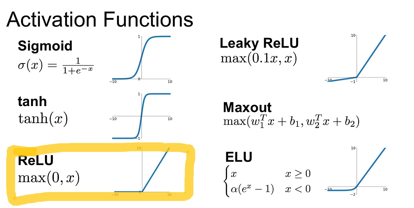
In Neural Network Basics: Part 2, the parameters of a function were found (optimised) to Minimise the Loss Function. The Loss Function chosen was the Mean Absolute Error, it could have been chosen to be the Mean Squared Error.

But What is the mathematical function if the wish to model something more complex like predicting the breed of Cat?

Unfortunately, its unlikely the relationship between the parameters and whether a pixel is part of a Maine Coon 🐈 is a Quadratic, its going to be something more complicated.

Thankfully, there exists the infinitely flexible function known as Rectified Linear Unit (ReLU)

1. Rectified Linear Unit (ReLU)

from ipywidgets import interact
from fastai.basics import *
from functools import partial

1.1 Function

The function does two things:
1. Calculate the output of a line
2. If the output is smaller than zero, return zero

def rectified_linear(m,b,x):
    y = m*x+b
    return torch.clip(y,0.)

1.2 Create A Custom ReLU Method

def custom_relu_fn(m,b): return partial(rectified_linear,m,b)

1.3 Create `y = 1x + 1` with Custom ReLU Method

fn_11 = custom_relu_fn(1,1)
fn_11

functools.partial(<function rectified_linear at 0x00000220331C9D00>, 1, 1)

1.4 ReLU `y = 1x+ 1` Plot

x = torch.linspace(-2.1,2.1,20)
plt.plot(x,fn_11(x))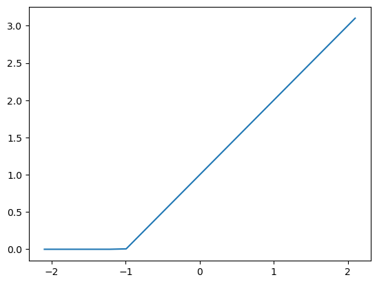

1.4.1 Interactive ReLU

plt.rc('figure', dpi=90)

@interact(m=1.2, b=1.2)
def plot_relu(m, b):
    min, max = -4.1, 4.1
    x = torch.linspace(min,max, 100)[:,None]
    fn_fixed = partial(rectified_linear, m,b)
    ylim=(-1,4)
    plt.ylim(ylim)
    plt.axvline(0, color='gray', linestyle='dotted', linewidth=2)
    plt.axhline(0, color='gray', linestyle='dotted', linewidth=2)
    plt.plot(x, fn_fixed(x))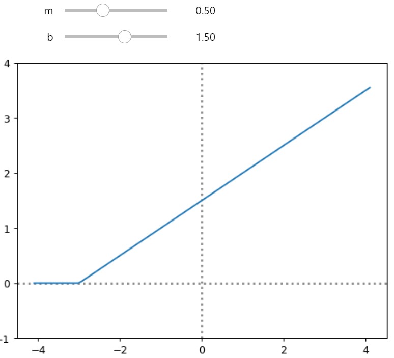

1.5 Double ReLU Function

def double_relu(m1,b1,m2,b2,x):
    return rectified_linear(m1,b1) + rectified_linear(m2,b2)

1.5.1 Interactive Double ReLU

plt.rc('figure', dpi=90)

def dbl_rectified_linear(m1, b1,m2,b2,x): 
    return rectified_linear(m1,b1,x) + rectified_linear(m2,b2,x)
 
@interact(m1=-1.2, b1=-1.2,m2=1.2, b2=1.2)
def plot_dbl_relu(m1,b1,m2,b2):
    min, max = -3.1, 3.1
    x = torch.linspace(min,max, 100)[:,None]
    fn_fixed = partial(dbl_rectified_linear, m1,b1,m2,b2)
    ylim=(-1,4)
    xlim=(-4,4)
    plt.ylim(ylim)
    plt.xlim(xlim)
    plt.axvline(0, color='gray', linestyle='dotted', linewidth=2)
    plt.axhline(0, color='gray', linestyle='dotted', linewidth=2)
    plt.plot(x, fn_fixed(x))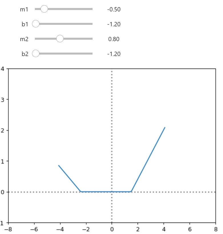

1.5.1 Triple ReLU for Good Measure!

def trple_rectified_linear(m1, b1, m2, b2, m3, b3, x): 
    return rectified_linear(m1,b1,x) + rectified_linear(m2,b2,x) + rectified_linear(m3,b3,x)
 
@interact(m1=-1.2, b1=-1.2,m2=1.2, b2=1.2, m3=0.5, b3=0.5)
def plot_trple_relu(m1,b1,m2,b2,m3,b3):
# static variables
    min, max = -3.1, 3.1
    x = torch.linspace(min,max, 100)[:,None]
    
# update partial to include extra parameters m3, b3
    triple_relu_fn_y = partial(trple_rectified_linear, m1,b1,m2,b2,m3,b3)

# static variables
    ylim=(-1,4) 
    xlim=(-4,4)
    plt.ylim(ylim)
    plt.xlim(xlim)
    plt.axvline(0, color='gray', linestyle='dotted', linewidth=2)
    plt.axhline(0, color='gray', linestyle='dotted', linewidth=2)
    plt.plot(x, triple_relu_fn_y(x))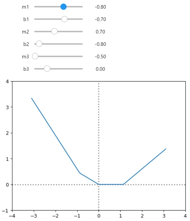

2. ReLU is An Infinitely Flexible Function

There could be arbitrarily many ReLus added together to form any function!

The previous functions are of a single input x i.e. 2-Dimensions.

ReLU’s could be added together over as many dimensions as desired, i.e. ReLU’s over surfaces or ReLU’s over 3D, 4D 5D etc.

But adding these ReLU’s, this means there are arbitrary amount of parameters related to each ReLU, how can these parameters be calculated?

In Part 2, a optimisation method called Gradient Descent was used to determine Parameters.

That’s Deep Learning in a nutshell. Beyond this, Tweaks are to:
- make it faster
- require less data

Neural Network Basics Completed.

Go back to a previous post:

Neural Network Basics: Part 1
Neural Network Basics: Part 2
Neural Network Basics: Part 3